---
title: "Chapter 1: The Sample Space"
subtitle: "Feller — Probability Theory and Its Applications"
date: 2026-01-02
toc: true
toc-depth: 3
number-sections: true
bibliography: ../../references.bib
---
## Events and Sample Spaces
Consider an experiment whose possible outcomes form a **sample space** $\Omega$. Each outcome is a point in $\Omega$, and any subset of $\Omega$ is called an **event**.
::: {#def-events}
## Events
Given events $A$ and $B$ in a sample space $\Omega$:
- $AB = A \cap B$ is the event that both $A$ and $B$ occur.
- $A \cup B$ is the event that at least one of $A$, $B$ occurs.
- $A$ and $B$ are **mutually exclusive** if $AB = \emptyset$.
- $A \subset B$ means every outcome in $A$ is also in $B$ ($A$ implies $B$).
- $A - B$ is the event that $A$ occurs but $B$ does not.
- $\bar{A} = \Omega - A$ is the **complement** of $A$.
:::
::: {#def-probability}
## Probability on a Discrete Space
Given a discrete sample space $\Omega = \{E_1, E_2, \ldots\}$, a **probability measure** is an assignment of non-negative numbers $\mathbb{P}(E_j)$ to each sample point satisfying
$$\mathbb{P}(E_1) + \mathbb{P}(E_2) + \cdots = 1.$$
The probability of an event $A \subset \Omega$ is
$$\mathbb{P}(A) = \sum_{E_j \in A} \mathbb{P}(E_j).$$
:::
::: {.callout-tip collapse="true"}
## Example — Two coin flips
Let $\Omega = \{HH, HT, TH, TT\}$ with each outcome equally likely. Set $A$ = heads on the first toss, $B$ = tails on the second toss.
| Event | Elements | $\mathbb{P}$ |
|-------|----------|------|
| $A$ | $\{HH, HT\}$ | $1/2$ |
| $B$ | $\{HT, TT\}$ | $1/2$ |
| $AB$ | $\{HT\}$ | $1/4$ |
| $A \cup B$ | $\{HH, HT, TT\}$ | $3/4$ |
Note $\mathbb{P}(A \cup B) = \mathbb{P}(A) + \mathbb{P}(B) - \mathbb{P}(AB) = 1/2 + 1/2 - 1/4 = 3/4$.
:::
---
## Combinatorial Analysis
### Permutations
Consider a population of $n$ distinct elements. An **ordered sample** of size $r$ drawn from the population can be selected in:
- $n^r$ ways **with replacement**,
- $(n)_r = n(n-1)\cdots(n-r+1)$ ways **without replacement**.
When $r = n$, an ordered selection without replacement is a **permutation** of the full set:
$$(n)_n = n! = n(n-1)\cdots 2 \cdot 1.$$
::: {.callout-tip collapse="true"}
## Example — Five distinct digits
What is the probability that five digits drawn independently and uniformly from $\{0,\ldots,9\}$ are all different?
The total number of outcomes is $10^5$. The number of outcomes with all digits distinct is $(10)_5 = 10 \cdot 9 \cdot 8 \cdot 7 \cdot 6 = 30240$. Thus
$$\mathbb{P}(\text{all distinct}) = \frac{30240}{100000} = 0.3024.$$
:::
### The Birthday Problem {#sec-birthday}
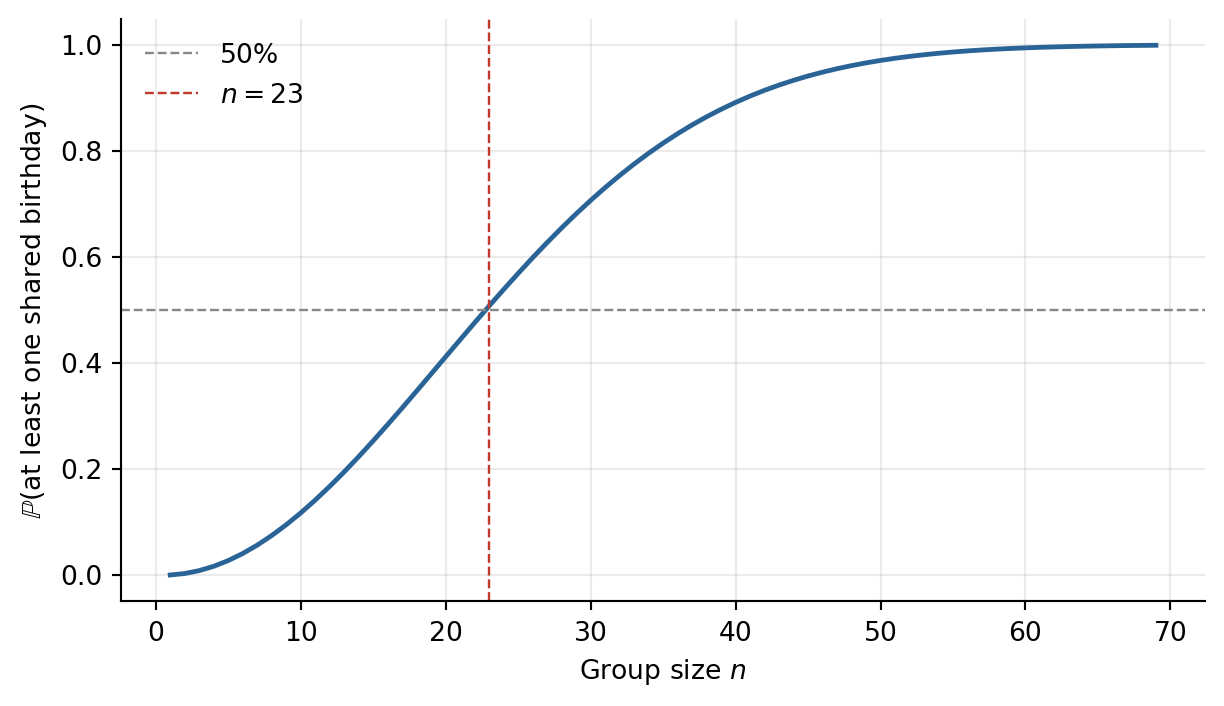
What is the probability that in a group of $n$ people, at least two share a birthday? Treating all 365 days as equally likely and ignoring leap years, the probability that **no two** share a birthday is
$$p_{\text{no match}} = \frac{(365)_n}{365^n} = \prod_{k=0}^{n-1}\left(1 - \frac{k}{365}\right).$$
For small $n$, dropping terms of order $(1/365)^2$:
$$p_{\text{no match}} \approx 1 - \frac{n(n-1)}{730},$$
so $\mathbb{P}(\text{at least one match}) \approx n(n-1)/730$. For larger $n$, taking logs and using $\log(1-x)\approx -x$:
$$p_{\text{no match}} \approx e^{-n(n-1)/730}.$$
The crossover point $p_{\text{match}} \geq 1/2$ occurs at $n = 23$.
```{python}
#| label: fig-birthday
#| fig-cap: "Probability of at least one shared birthday vs. group size."
#| code-fold: true
import numpy as np
import matplotlib.pyplot as plt

n_vals = np.arange(1, 70)
p_no_match = np.array([np.prod([(365-k)/365 for k in range(n)]) for n in n_vals])
p_match = 1 - p_no_match

fig, ax = plt.subplots(figsize=(6.5, 3.8))
ax.plot(n_vals, p_match, color='#2a6496', linewidth=1.8)
ax.axhline(0.5, color='#888', linestyle='--', linewidth=0.9, label='50%')
ax.axvline(23, color='#c0392b', linestyle='--', linewidth=0.9, label='$n=23$')
ax.set_xlabel('Group size $n$')
ax.set_ylabel('$\\mathbb{P}$(at least one shared birthday)')
ax.legend(frameon=False)
ax.grid(True, alpha=0.25)
ax.spines[['top','right']].set_visible(False)
plt.tight_layout()
plt.show()
```
### Combinations
::: {#thm-binomial}
## Binomial Coefficient
The number of unordered subsets of size $r$ drawn from $n$ elements is
$$\binom{n}{r} = \frac{(n)_r}{r!} = \frac{n!}{r!\,(n-r)!}.$$
:::
::: {.proof}
From $n$ elements we can form $(n)_r$ ordered samples of size $r$. Each unordered subset of size $r$ appears exactly $r!$ times among these (once for each ordering of its elements), so the number of unordered subsets is $(n)_r / r!$.
:::
::: {.callout-tip collapse="true"}
## Example — $\binom{5}{3} = 10$
We want unordered groups of 3 from $\{1,2,3,4,5\}$. There are $5! = 120$ total orderings of all five elements. Each group of 3 appears in $3! = 6$ orderings among the first three positions, and the remaining $2! = 2$ orderings of the last two positions are irrelevant. So
$$\binom{5}{3} = \frac{5!}{3!\cdot 2!} = \frac{120}{12} = 10.$$
:::
::: {#thm-binomial-theorem}
## Binomial Theorem
For any real $x, y$ and non-negative integer $n$,
$$(x + y)^n = \sum_{k=0}^{n} \binom{n}{k} x^k y^{n-k}.$$
:::
Setting $x = y = 1$ gives $\sum_{k=0}^n \binom{n}{k} = 2^n$, the total number of subsets of an $n$-element set.
---
## Problem Set
### Core Problems (Feller)
**Problem 1.1.** Among the digits $1, 2, 3, 4, 5$ first one is chosen, and then a second from the remaining four. Assume all twenty outcomes equally likely. Find the probability that an odd digit is selected (a) first; (b) second; (c) both times.
::: {.callout-caution collapse="true"}
## Solution
Write out the $5 \times 4 = 20$ ordered pairs. The odd digits are $\{1, 3, 5\}$.
(a) Outcomes with an odd first digit: $3 \times 4 = 12$, so $\mathbb{P} = 12/20 = 3/5$.
(b) By symmetry, each position is equally likely to take any value, so $\mathbb{P}(\text{second odd}) = 3/5$.
(c) Both odd: choose the first odd in 3 ways, the second in 2 ways, giving $3 \times 2 = 6$ outcomes. $\mathbb{P} = 6/20 = 3/10$.
:::
**Problem 1.2.** A coin is tossed until the same result appears twice in succession. Assign probability $1/2^n$ to each outcome requiring $n$ tosses. (a) Describe the sample space. (b) Find $\mathbb{P}(\text{ends before toss 6})$. (c) Find $\mathbb{P}(\text{even number of tosses})$.
::: {.callout-caution collapse="true"}
## Solution
The sample space consists of strings of length $n \geq 2$ where the first $n-2$ characters alternate ($HTH\ldots$ or $THT\ldots$) and the last two are identical. For each $n$ there are exactly 2 outcomes, each with probability $1/2^n$.
**(b)** Sum over $n \in \{2,3,4,5\}$:
$$2\!\left(\frac{1}{4}+\frac{1}{8}+\frac{1}{16}+\frac{1}{32}\right) = \frac{30}{32} = \frac{15}{16}.$$
**(c)** Sum over even $n = 2, 4, 6, \ldots$:
$$2\sum_{k=1}^{\infty}\frac{1}{4^k} = 2 \cdot \frac{1/4}{1-1/4} = \frac{2}{3}.$$
:::
**Problem 1.3.** Two dice are thrown. Let $A$ = sum is odd, $B$ = at least one ace. Find $\mathbb{P}(AB)$, $\mathbb{P}(A \cup B)$, $\mathbb{P}(A\bar{B})$ assuming all 36 outcomes equally likely.
::: {.callout-caution collapse="true"}
## Solution
$\mathbb{P}(A) = 18/36 = 1/2$. For $B$: there are $6 + 6 - 1 = 11$ outcomes with at least one ace, so $\mathbb{P}(B) = 11/36$. The outcomes in $AB$ (odd sum and at least one ace) are $(1,2),(1,4),(1,6),(2,1),(4,1),(6,1)$, giving $\mathbb{P}(AB) = 6/36$.
$$\mathbb{P}(A \cup B) = \tfrac{18}{36} + \tfrac{11}{36} - \tfrac{6}{36} = \frac{23}{36}, \qquad \mathbb{P}(A\bar{B}) = \mathbb{P}(A) - \mathbb{P}(AB) = \frac{12}{36} = \frac{1}{3}.$$
:::
---
### Quant Finance Problems
**QF-1 — Gambler's Ruin.** A trader starts with \$3 and makes fair \$1 bets, stopping at \$0 or \$6.
(a) Find her probability of ruin using $p_k = 1 - k/N$.
(b) For unfair bets with win probability $p \neq 1/2$, the ruin probability from stake $k$ with target $N$ is $\bigl[(q/p)^k - (q/p)^N\bigr] / \bigl[1 - (q/p)^N\bigr]$ where $q = 1-p$. Compute for $p = 0.45$.
(c) What does this say about trading without edge?
**QF-2 — CRR Binomial Model.** Stock $S_0 = 100$, $u = 1.1$, $d = 0.9$, 3 periods, $r = 0$.
(a) Enumerate all 8 paths.
(b) Find $\mathbb{P}(S_3 > 105)$ under real-world $p = 0.6$.
(c) Find the risk-neutral probability $\tilde{p}$ satisfying $\tilde{p}\,u + (1-\tilde{p})\,d = 1$ and recompute.
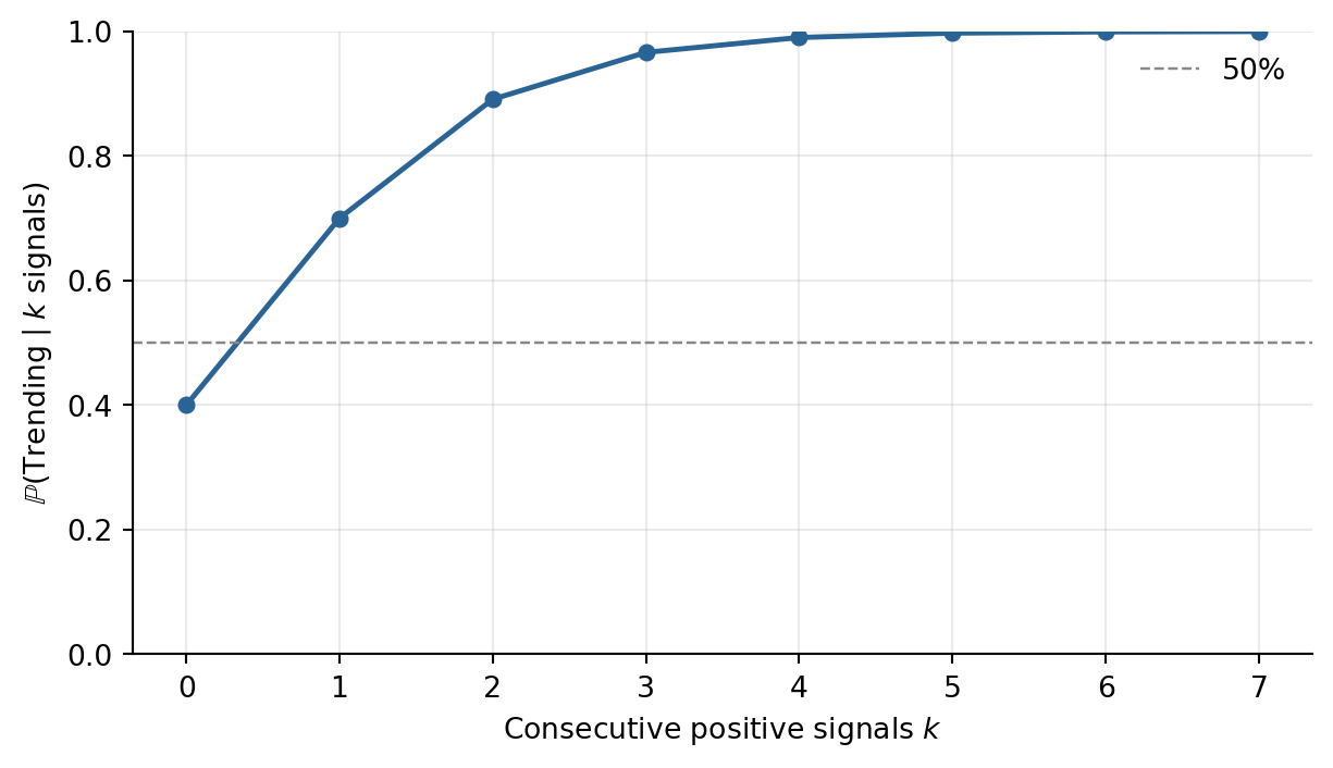
**QF-3 — Bayesian Regime Detection.** Prior $\mathbb{P}(\text{trending}) = 0.4$. A momentum signal fires on 70% of trending days and 20% of mean-reverting days.
(a) Posterior after one signal. (b) After two signals. (c) Prior needed for 50% posterior after one signal.
```{python}
#| label: fig-bayes-update
#| fig-cap: "Posterior probability of trending regime after $k$ consecutive positive signals."
#| code-fold: true
import numpy as np
import matplotlib.pyplot as plt

p_T, p_s_T, p_s_M = 0.4, 0.70, 0.20

posteriors, prior = [], p_T
for _ in range(8):
    posteriors.append(prior)
    prior = (prior * p_s_T) / (prior * p_s_T + (1 - prior) * p_s_M)

fig, ax = plt.subplots(figsize=(6.5, 3.8))
ax.plot(range(8), posteriors, 'o-', color='#2a6496', linewidth=1.8, markersize=5)
ax.axhline(0.5, color='#888', linestyle='--', linewidth=0.9, label='50%')
ax.set_xlabel('Consecutive positive signals $k$')
ax.set_ylabel('$\\mathbb{P}(\\text{Trending} \\mid k\\ \\text{signals})$')
ax.set_ylim(0, 1)
ax.legend(frameon=False)
ax.grid(True, alpha=0.25)
ax.spines[['top','right']].set_visible(False)
plt.tight_layout()
plt.show()
```