Two Quick Applications of Eigenvalues and Eigenvectors
Aside from their geometric interpretation, eigenvalues and eigenvectors provide convenient algebraic properties that can be used to solve interesting problems. Consider the following examples taken from Strang’s lectures in 18.06. He walks through two examples, one on Markov matrices and one on the Fibonacci numbers, and details how eigenvalues and eigenvectors can be used to understand long term behaviour. Below we outline both problems and provide a numerical implementation for each.
Sections
- Discrete Time Markov Chain
- Fibonacci Sequence
References
- Introduction to Linear Algebra by G. Strang (Chpt 6.1 & 6.2)
Discrete Time Markov Chain
Consider a two state DTMC with the following one-step transition matrix
\[P = \begin{bmatrix} 0.8 & 0.6 \\ 0.2 & 0.4 \end{bmatrix}\]Notice that each entry is non-negative and the sum of each column is 1. This matrix could be used to describe a very basic population model in which people travel between states according to the probabilities defined above. We want to understand the long term behaviour of this model. In section 1.1 we solve this problem using eigenvectors and eigenvalues and confirm our result experimentally, with a Monte Carlo simulation.
Theory
The dynamics of the population can formulated according the following first order recurrence
\[\mathbf{u}_{n+1} = P\mathbf{u}_{n}\]where $\mathbf{u}_n$ records the population percentage after $n$ iterations, with $\mathbf{u}_0$ defining the initial distribution. It is easy to come up with a closed form solution to this recurrence by repeated substitution
\[\begin{align*} \mathbf{u}_1 &= P\mathbf{u}_0\\ \mathbf{u}_2 &= P\mathbf{u}_1\\ &=P(P\mathbf{u}_0) = P^2\mathbf{u}_0\\ \vdots\\ \mathbf{u}_k &= P^k\mathbf{u}_0 \end{align*}\]Thus we are interested in finding $P^k$. We could solve for iteration $k$ by simply applying matrix multiplication $k$ times, but for any reasonably large $k$ that becomes unfeasible. We seek a better way using eigenvalues and eigenvectors. Recall that an eigenvector, $x$, of the matrix $P$ is defined as \(Px = \lambda x\) meaning the application of $P$ to the vector $x$ scales the vector by a factor of $\lambda$. To find eigenvectors we can rearrange the above relation
\[Px = \lambda x\iff (P-\lambda I)x = \mathbf{0}\iff det(P-\lambda I) = 0\]Since we are dealing with a Markov matrix we know $\lambda_1=1$ (realize $P-I$ is always singular for any Markov matrix $P$) and the other must satisfy
\[tr(P) = 0.8 + 0.4 = 1.2 = \lambda_1+\lambda_2 \implies \lambda_2 = 0.2\]Now that we have both eigenvalues we seek their corresponding eigenvectors, that is we want to find the Null Space of
\[P-I = \begin{bmatrix} 0.8 - 1 & 0.6 \\ 0.2 & 0.4 - 1 \end{bmatrix} \implies \begin{bmatrix} -0.2 & 0.6 \\ 0.2 & -0.6 \end{bmatrix}\begin{bmatrix}3 \\1\end{bmatrix} = \mathbf{0}\] \[P-0.2I = \begin{bmatrix} 0.8 - 0.2 & 0.6 \\ 0.2 & 0.4 - 0.2 \end{bmatrix} \implies \begin{bmatrix} 0.6 & 0.6 \\ 0.2 & 0.2 \end{bmatrix}\begin{bmatrix}1 \\-1\end{bmatrix} = \mathbf{0}\]So, we have eigenvalues $\lambda_1 =1, \lambda_2=0.2$ and corresponding eigenvectors
\[\mathbf{x}_1 = \begin{bmatrix}3 \\ 1\end{bmatrix}, \mathbf{x}_2 = \begin{bmatrix}1 \\ -1\end{bmatrix}\]The useful thing about these quantities is that if we can write our initial condition as some combination of eigenvectors we can simplify the matrix exponential considerably
\[\begin{align*} \mathbf{u}_k &= P^k\mathbf{u}_0\\ &= P^k(c_1\mathbf{x}_1 + c_2\mathbf{x}_2)\\ &= c_1P^k\mathbf{x}_1 + c_2P^k\mathbf{x}_2\\ &= c_1\lambda_1^k \mathbf{x}_1 + c_2\lambda_2^k\mathbf{x_2} \end{align*}\]For the initial distribution let’s imagine that $70\%$ of all people start in location 1 and the remaining $30\%$ start in the other location. Then we can rewrite
\[\mathbf{u}_0 = \begin{bmatrix} 0.7 \\ 0.3\end{bmatrix} = 0.25\begin{bmatrix} 3 \\ 1\end{bmatrix} - 0.05\begin{bmatrix} 1 \\ -1\end{bmatrix}\]and so, the long term behavior is defined by the following relation
\[\begin{align*} \mathbf{u}_k &= P^k\mathbf{u}_0\\ &= c_1\lambda_1^k \mathbf{x}_1 + c_2\lambda_2^k\mathbf{x_2}\\ &= 0.25(1)^k\begin{bmatrix} 3 \\ 1\end{bmatrix} - 0.05(0.2)^k\begin{bmatrix} 1 \\ -1\end{bmatrix} \end{align*}\]and we can see that in the limit, as $k\rightarrow \infty$, the second term disappears and we are left with the following distribution of people
\[\begin{bmatrix}3/4 \\ 1/4\end{bmatrix}\]import numpy as np
from numpy import linalg as LA
import matplotlib.pyplot as plt
plt.style.use('fivethirtyeight')
# one-step transition matrix
P = np.array([[0.8, 0.6],
               [0.2, 0.4]])

# determine eigenvalues/vectors
e_vals, e_vecs = LA.eig(P)
print('Eigenvalues: {}, {}\nEigenvector 1: {}\nEigenvector 2 {}'.format(e_vals[0], e_vals[1], e_vecs[0], e_vecs[1]))

# set the initial condition 70/30 split
IC = np.array([[0.7], [0.3]])

# determine coefficients c_1, c_2 so that
# IC can be written as linear combination
# of eigenvectors
c = LA.inv(e_vecs)@IC
k=5000

u_k = c[0]*(e_vals[0]**k)*e_vecs[:, 0] + c[1]*(e_vals[1]**k)*e_vecs[:, 1]
print('Long term distribution: {}'.format(u_k))
Eigenvalues: 1.0, 0.20000000000000007
Eigenvector 1: [ 0.9486833  -0.70710678]
Eigenvector 2 [0.31622777 0.70710678]
Long term distribution: [0.75 0.25]
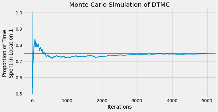
Notice that the eigenvectors evaluated using numpy are not the same as the ones found above. This is not a problem as they are identical up to a constant multiple; there are many eigenvectors we could have chosen. In the end, we find that at $k=5000$ iterations we see the long term distribution we expected. Below is a simple Monte Carlo simulation that will iterate transitions between states according the probability distribution defined by $\mathbf{P}$ for $k=5000$ time steps. We keep track of the proportion of times the existing state is location 1. The red line below is marked at 0.75 and we see that convergence happens rather quickly after about 1000 iterations, confirming what we found above.
pi0 = np.array([0, 1])
state = np.random.choice([0, 1], p=P@pi0)

proportion_list = []
count_d = {'0':0, '1':0}
i=0
while i < k:
    state = np.random.choice([0, 1], p=P[:, state])
    count_d[str(state)]+=1
    i+=1
    proportion_list.append(count_d['0']/i)
count_d['0']/sum(count_d.values())

fig, ax = plt.subplots(figsize=(10, 5))
plt.plot([i for i in range(k)], proportion_list, lw=2)
plt.axhline(y=0.75, color='r', linestyle='-', lw=2)
plt.xlabel('Iterations')
plt.ylabel('Proportion of Time\nSpent in Location 1')
plt.title('Monte Carlo Simulation of DTMC');
Fibonacci Numbers
Now we take a look at how eigenvalues and eigenvectors can help us define Fibonacci numbers. Recall the Fibonacci sequence for the $n$th Fibonacci Number
\[F_n = F_{n-1}+F_{n-2},\quad n\geq 2\]where $F_0 = 0, F_1=1$. This is a second order recurrence relation that we can turn it into a first order system by taking \(\mathbf{u}_n = \begin{bmatrix} F_n \\ F_{n-1}\end{bmatrix}\) and noticing
\[\underbrace{\begin{bmatrix}F_n \\ F_{n-1}\end{bmatrix}}_{\mathbf{u}_n} = \underbrace{\begin{bmatrix}1 & 1\\ 1 & 0 \end{bmatrix}}_{A}\underbrace{\begin{bmatrix}F_{n-1} \\F_{n-2}\end{bmatrix}}_{\mathbf{u}_{n-1}},\quad n\geq 2\]In the same vein as the DTMC we can study the long term behaviour of this recurrence by evaluating $A^k\mathbf{u}_{n-1}$. In particular, $A^k$ will give is the information to find the $k$th Fibonacci number and studying it’s eigenvectors will give us an idea of how they grow. That being said, we wish to find the roots of the characteristic polynomial
\[\lambda^2 - \lambda -1 =0\]which, after using the quadratic formula, are found to be $\lambda=\frac{1\pm\sqrt{5}}{2}$. The corresponding eigenvectors are not difficult to find,
\[x_1 = \begin{bmatrix}1 + \sqrt{5} \\ 2\end{bmatrix}, x_2 = \begin{bmatrix}1-\sqrt{5} \\ 2\end{bmatrix}\]Now we want to write the initial condition \(\mathbf{u}_1 = \begin{bmatrix}1 \\ 0\end{bmatrix}\) as a sum of the eigenvectors. This amounts to finding $\mathbf{c}$ such that
\[\begin{bmatrix}1 \\ 0 \end{bmatrix} = \begin{bmatrix}1+\sqrt{5} & 1-\sqrt{5} \\ 2 & 2\end{bmatrix}\begin{bmatrix}c_1 \\ c_2\end{bmatrix}\implies \begin{bmatrix}c_1 \\ c_2\end{bmatrix} = \begin{bmatrix}1+\sqrt{5} & 1-\sqrt{5} \\ 2 & 2\end{bmatrix}^{-1}\begin{bmatrix}1 \\ 0 \end{bmatrix}\]solving this we find
\[\mathbf{c} = \begin{bmatrix}\frac{1}{2\sqrt{5}}\\ -\frac{1}{2\sqrt{5}}\end{bmatrix}\]and so, the long term behaviour is characterised by
\[\begin{align*} \mathbf{u}_k &= P^k\mathbf{u}_0\\ &= c_1\lambda_1^k \mathbf{x}_1 + c_2\lambda_2^k\mathbf{x_2}\\\\ &= \frac{1}{2\sqrt{5}}\left(\frac{1+\sqrt{5}}{2}\right)^k\begin{bmatrix}1+\sqrt{5} \\ 2 \end{bmatrix} -\frac{1}{2\sqrt{5}}\left(\frac{1-\sqrt{5}}{2}\right)^k \begin{bmatrix}1-\sqrt{5} \\ 2\end{bmatrix}\\\\ &= \frac{1}{\sqrt{5}}\left(\frac{1+\sqrt{5}}{2}\right)^k\begin{bmatrix}\frac{1+\sqrt{5}}{2} \\ 1 \end{bmatrix} -\frac{1}{\sqrt{5}}\left(\frac{1-\sqrt{5}}{2}\right)^k \begin{bmatrix}\frac{1-\sqrt{5}}{2} \\ 1\end{bmatrix} \end{align*}\]Notice that we can extract the $k$th Fibonacci number using the second component of both $x_1$ and $x_2$. This means that
\[F_k = \frac{1}{\sqrt{5}}\left(\left(\frac{1+\sqrt{5}}{2}\right)^k - \left(\frac{1-\sqrt{5}}{2}\right)^k\right)\]Moreover, the second term
\[\frac{1-\sqrt{5}}{2}\approx -0.618\]disappears in the limit as $k\rightarrow\infty$. Also notice that the Fibonacci rule is always defined as the sum of two integers, $F_{n-1}$ and $F_{n-2}$, which means that the $k$th Fibonacci number is always the closest integer to
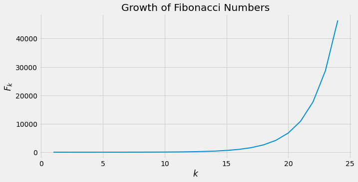
\[\frac{1}{\sqrt{5}}\left(\frac{1+\sqrt{5}}{2}\right)^k\]Below we use the relation for $F_k$ to display the first 50 Fibonacci number and look at their growth.
fig, ax = plt.subplots(figsize=(10, 5))
def k_fib(k):
    return int(round(1/np.sqrt(5)*((1+np.sqrt(5))/2)**k))
x = np.arange(1, 25)
fibs = list(map(k_fib, x))
for i in range(26):
    print('k={}, F_k={}'.format(i, k_fib(i)))
plt.plot(x, fibs, lw=2)
plt.title('Growth of Fibonacci Numbers')
plt.xlabel('$k$')
plt.ylabel('$F_k$');
k=0, F_k=0
k=1, F_k=1
k=2, F_k=1
k=3, F_k=2
k=4, F_k=3
k=5, F_k=5
k=6, F_k=8
k=7, F_k=13
k=8, F_k=21
k=9, F_k=34
k=10, F_k=55
k=11, F_k=89
k=12, F_k=144
k=13, F_k=233
k=14, F_k=377
k=15, F_k=610
k=16, F_k=987
k=17, F_k=1597
k=18, F_k=2584
k=19, F_k=4181
k=20, F_k=6765
k=21, F_k=10946
k=22, F_k=17711
k=23, F_k=28657
k=24, F_k=46368
k=25, F_k=75025